今天经验啦给大家讲解Excel图表次坐标轴添加方法内容,有需要或者有兴趣的朋友们可以看一看下文,相信对大家会有所帮助的 。
Excel图表次坐标轴添加方法内容

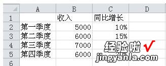
1、打开所要建立图表的Excel工作表,数据对照设计 。
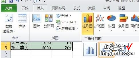
2、全选数据 , 点击插入柱形图;
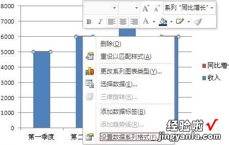
3、右键红色柱形图(即同比增长数据)选择‘设置数字系列格式’
4、选择次坐标轴
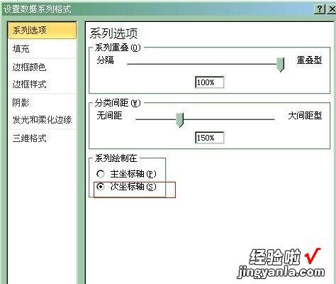
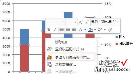
5、右边出现次坐标轴,由于图表感觉不美观,右键红色图表选择‘更改系列图表类型’
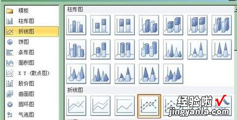
6、选择折线图中红色选择图表类型
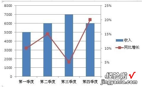
7、此时要建立的图表结构已经形成,增加数值的显示更加贴切
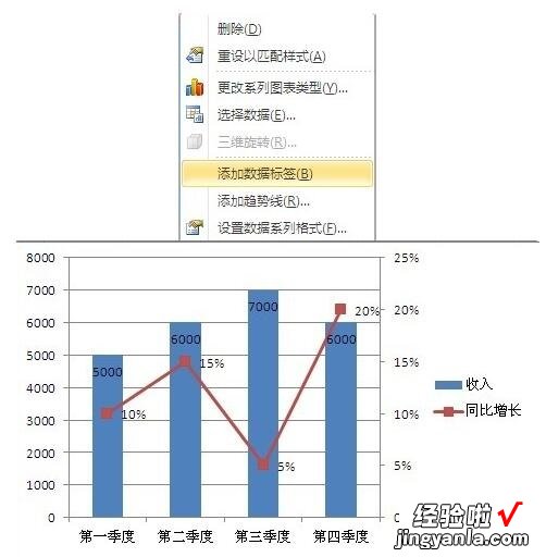
8、右键柱形图和折线图选择‘添加数据标签’,调整下数值的位置就显示完整的图表了
【分享Excel图表次坐标轴添加方法内容】
学完本文Excel图表次坐标轴添加方法,是不是觉得以后操作起来会更容易一点呢?